How to create your own functions in R

We’ve talked a lot about how to use different pre-made functions in R, but sometimes you just need to make your own function to tackle your data. In this blog post, I’m going to talk about how to create your own function and give a few examples.

Components of a function

Remember that a function is essentially a “black box” into which you add some inputs and then receive some outputs. Building a function is about building that “black box”, and there are several components that go into it.

Let’s first discuss those components. I’ve created an example function below, called “add_three”. It adds three to the value that is passed by the user.

add_three <- function(x){
  y <- x + 3
  return(y)
}

add_three(5)

## [1] 8

Take note of a few important elements:

• Function name (add_three): this is just the name that you want to call your function. It should be something pretty short and easy to remember, like so many of the common functions we use (e.g., mean, plot, select). I chose the name “add_three”. As when we create any variables or objects in R, we use the arrow <- to assign this name to our function.

• “function” and arguments (function(x)): we tell R that we want to create a function using function(). Within the parentheses, we can specify the number of arguments that we want our function to have. It doesn’t matter what we name our arguments within the parentheses (I named mine x), as long as we use the same names in the body of the function. If you want to have multiple arguments, it would look something like this: function(arg1, arg2, arg3, ...). Later, when you put your function to use, you’ll have to specify values for the arguments, like I did with the 5 in add_three(5).

• Curly brackets: { and } come after function(argument) and need to bracket the actual function code that you’re writing.

• Body of the function: this is the code in the function between the curly brackets that executes the task that you want. Here, I’ve created a new variable, y, to store the x + 3 value.

• The return value (return(y)): Also inside the curly brackets, but usually at the end, this is the result that the function prints for you when it’s done running. I asked the function to return the value of y (aka, x + 3) to me.

And that’s all there is to creating your own function! Now I have a great function called add_three that I can use over and over again. You’ll notice that when you create a function, R adds this function to your environment. Just like you have to load packages to use them in a script, you’ll have to run your function code to add it to your environment each time you use it in a new script.

The example I just gave was very simple, but learning how to create your own function unlocks a whole new realm of coding that can be as simple or complex as you want.

A few examples

Mathematical formulas

It’s not that hard to add three to a value. In fact, we probably didn’t need to create a function for that. But what if we want to create a function that performs something more complex, like solving quadratic equations? Let’s create a quadratic formula function.

quadratic <- function(a, b, c){
  root1 <- (-b + sqrt(b^2 - 4 * a * c)) / (2 * a)
  root2 <- (-b - sqrt(b^2 - 4 * a * c)) / (2 * a)
  root1 <- paste("x =", root1)
  root2 <- paste("x =", root2)
  ifelse(root1 == root2, return(root1), return(c(root1, root2)))
}

This function accepts the coefficient \(a\) of the quadratic term, the coefficient \(b\) of the linear term, and the constant \(c\) as arguments. I created two values to hold the two possible roots of the equation. I also wanted the function to print “x = answer”, so I created values that pasted the “x =” string onto the answer. The ifelse statement at the end just says that if the two roots are equivalent, print only one of them. Otherwise, print both roots.

Now let’s see if the function works. Let’s test an equation with only one root, \(x^2 + 6x + 9 = 0\), and an equation with two roots: \(x^2 - 8x + 15 = 0\)

quadratic(1, 6, 9)

## [1] "x = -3"

quadratic(1, -8, 15)

## [1] "x = 5" "x = 3"

It works! And now we have a function to help with our math homework :)

Manipulating strings

Now that we’ve created a mathematical function, let’s try creating a function that manipulates strings. Let’s say we want a function that accepts a species name as an argument and returns an abbreviated version: the first letter of the genus + the rest of the species name. For example, the blue crab, Callinectes sapidus, would be shortened to C. sapidus.

shorten <- function(name){
  name_split <- strsplit(name, split = " ")
  genus <- substr(name, 1, 1)
  species <- name_split[[1]][2]
  new_name <- paste(genus, ". ", species, sep = "")
  print(new_name)
}

I first used strsplit() to split up the full species name into genus and species, by specifying that I wanted the split to occur at the space between the words. The function substr() allows you to pick out specific characters in a string. I asked substr() to just take the first letter of the name. Then I created the new string by pasting together the first letter of the genus, a period and space, and the species.

shorten("Homo sapiens")

## [1] "H. sapiens"

shorten("Leiostomus xanthurus")

## [1] "L. xanthurus"

Neat! This could be really useful for shortening the names in a list of species — writing a custom function makes the process much easier.

Functions without arguments

You can also create functions that don’t require arguments at all. For example, I could create a function that generates random coordinates for me, prints them, and plots them on a world map.

# Load necessary packages
library(tidyverse)
library(maps)

# Create the function
coords <- function(){
  # Randomly sample to get a random lat and long
  latitude <- runif(n = 1, min = -90, max = 90)
  longitude <- runif(n = 1, min = -180, max = 180)
  print(paste("Latitude: ", latitude, " Longitude: ", longitude, sep = ""))
  
  # get data to plot a world map 
  world <- map_data("world")

  # Plot the world map
  ggplot() +
    geom_map(data = world, map = world,
      aes(long, lat, map_id = region),
      color = "black", fill = "lightgray", size = 0.1) +
    # Plot our random point on top of the world map
    geom_point(aes(longitude, latitude), color = "red")
}

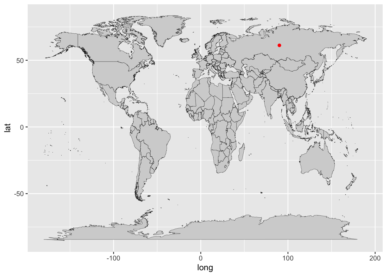
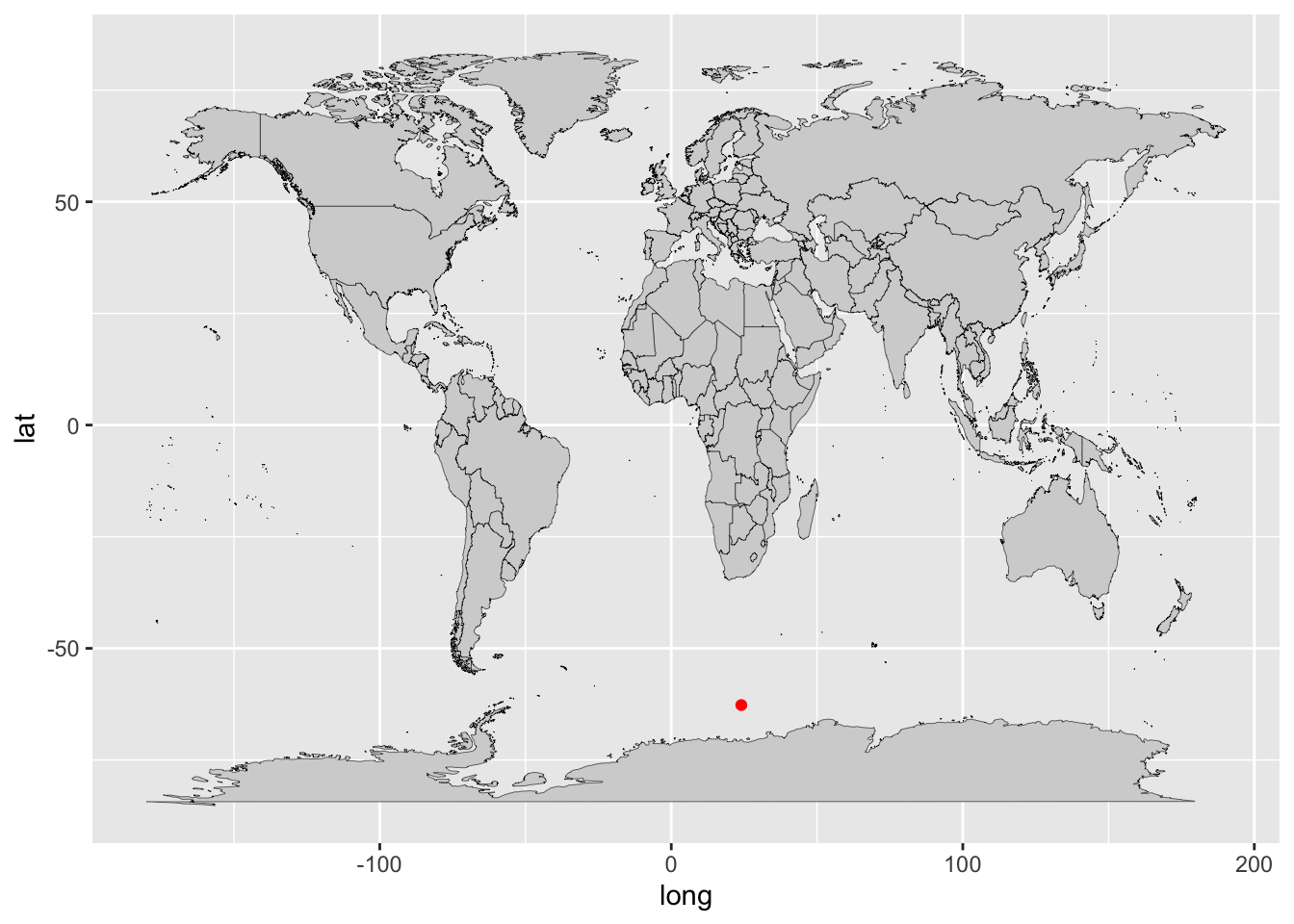
I used the runif() function to randomly sample one value each from the range of viable latitudes and longitudes. I used print() and paste() to display a message telling you the latitude and longitude values. Then I plotted the world map and our random point on top.

# What coordinates will I get this time?
coords()

## [1] "Latitude: 61.1949375551194 Longitude: 90.1810506172478"

# What about this time?
coords()

## [1] "Latitude: -62.7056198241189 Longitude: 24.0213383920491"

These examples were just three of many, many possibilities. Whatever task or operation you can think of in R, you can code it in a function. Get creative and have fun! Happy coding!

If you liked this and want learn more, you can check out the full course on the complete basics of R for ecology right here or by clicking the link below.