How to use R Markdown (part one)

Today I’m excited to share a blog post on how to use R Markdown. R Markdown is a dynamic file format that allows you to make documents containing normal text alongside chunks of embedded R code. In fact, all of my blog posts are written using R Markdown, which is how I’m able to write text like this, write code, and even insert a chunk of code

like_this <- c("isn't", "this", "neat?")

R Markdown is useful for several reasons:

• It’s great for reproducibility, where you can explain your analyses alongside your code and output so someone can follow along and replicate your work

• It helps with accountability, because all your code and the exact corresponding outputs are knit together into the final document

• It allows you to make tutorials like this one

• Finally, you can use it for learning R by helping you keep track of your notes and thinking process all while creating a custom reference document (more on this in part two!)

This tutorial is the first post of a two-part series on R Markdown. Here, you’ll learn how to create R Markdown documents with different types of content, and in part two I’ll go into how you can use it for learning R.

You can also follow along with this blog post in video format if you click on the image below. This post covers material in the video up to 35:35. I’ll cover the rest of the video in part two next week.

Getting set up with R Markdown

To use R Markdown, you’ll need to have R and RStudio already installed. If you need help with that, you can check out my blog post and lessons one, two, and three of my online course. These resources show you how to get started with R and RStudio.

You’ll also have to install two packages: rmarkdown and knitr. To do that you can run install.packages("rmarkdown") and install.packages("knitr"). You’ll only need to do this once for your computer (at least until the next time you update R).

install.packages("rmarkdown")
install.packages("knitr")

Now that you have the basic software and packages installed, you can get started with using R Markdown!

The first thing you’ll do after opening RStudio is go to File » New File » R Markdown.

Then a new window will pop up where you can fill out the title of your new document, the author (um, your name? 😉), and the output format. You can choose between HTML, PDF, and Word. We’re going to choose HTML for now, since that’s the simplest option and all you really need. Then hit OK.

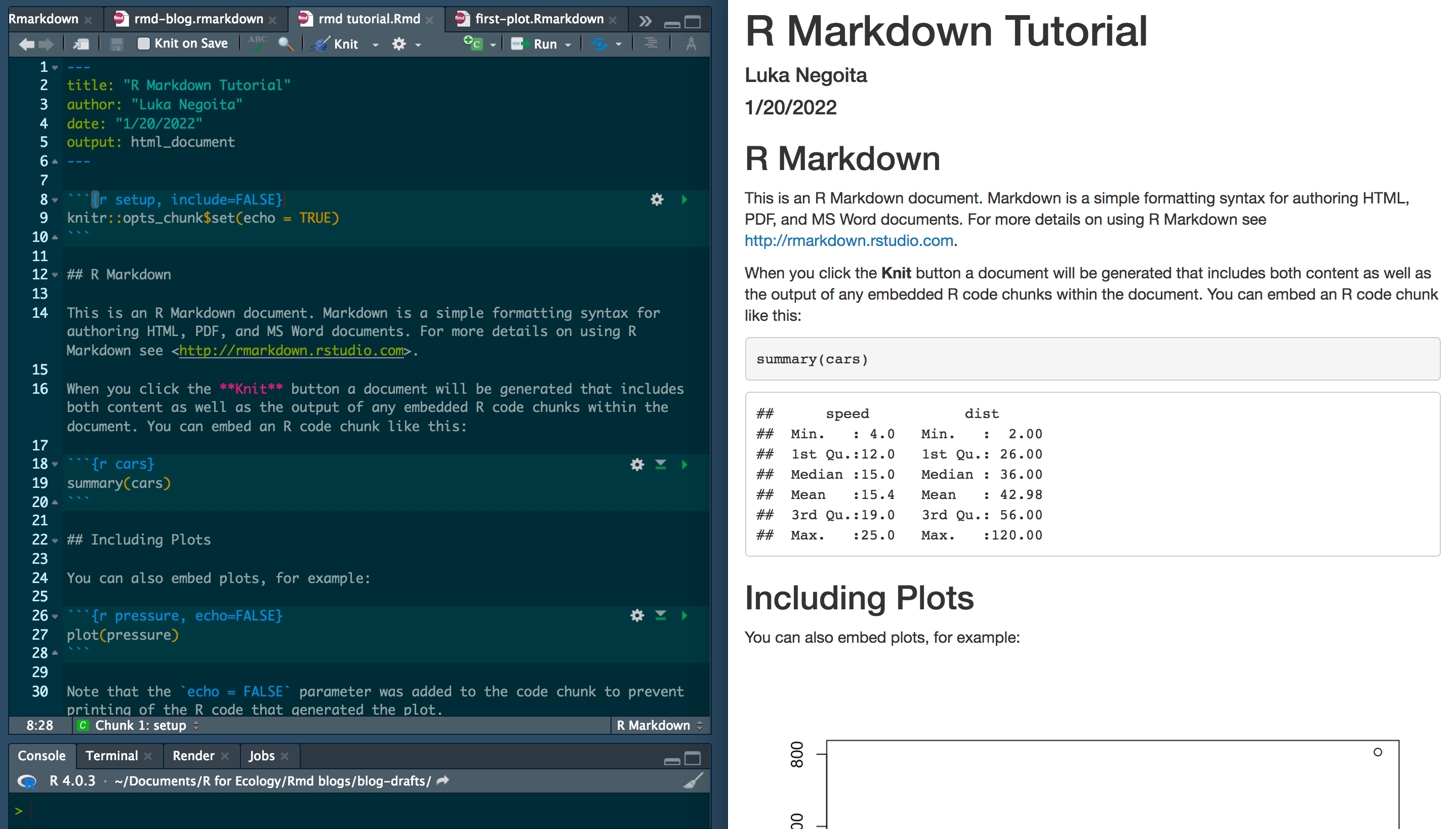
You’ll now have a new document that is filled in with a bunch of example content. At the top, in between the boundary lines (---), you’ll see a list of document parameters that should reflect what you entered in the previous window (title, author, output). You don’t need to change anything there. We’ll come back to this header section later.

The next section shows a code chunk that says “r setup”. This sets a bunch of code chunk parameters for the rest of the document. There’s no real need to include this, so we’ll delete it for now.

What you see now is the raw R Markdown content, which contains chunks of R code between chunks of regular text with Markdown formatting. But the true power of R Markdown is when you transform that text and code into a stand-alone document.

So how do we get from an R Markdown document in RStudio to the HTML document? You click on the “Knit” button (no need to click on the dropdown arrow). The lingo here is that the R Markdown document “knits” itself into an HTML document.

If you haven’t saved your document yet, you’ll be prompted to save it when you click “Knit”. You’ll notice that R Markdown files are saved as a .Rmd file instead of a .R file. Now that you’ve saved your document somewhere, it will automatically save itself every time you press “Knit” from now on.

The final HTML file will automatically display in the ‘Viewer’ panel (usually on the right).

If you explore the document a little, you can see that R Markdown really lets you do a lot. You can include different types of text formats, links, code chunks, and even plots.

Working on your own R Markdown document

Cool. Now let’s get started on creating our own R Markdown document. First let’s start with a blank slate. Go ahead and delete everything in the sample document so that all you have left is the parameter header. It’s important that you leave that in!

Try to type some text, whatever you want. If you press “Knit”, it should then show up in a knitted document, and your .Rmd file should be automatically saved. Anything you type will show up in the knitted document! Neat.

Learning R Markdown text formats

Now let’s explore different types of text formatting in R Markdown. To organize different sections of your report, you’ll want to add section headings or titles. You can write headings of different sizes by writing different numbers of pound signs (#) + a space + your text, like this:

As you can see, the more pound signs you add, the smaller the headings get.

You can also add bold and italicized text by surrounding text with asterisks (*). Using one asterisk gives you italicized text, using two gives you bold text, and using three gives you bold italicized text.

You can create numbered lists just using 1. 2. 3. (…) in front of your text.

And you can create bulleted lists using either hyphens (-) or asterisks (*) before your text.

You can add links by putting square brackets [these] around the word or phrase that you want to hyperlink, and then immediately put the link (with the https://) in parentheses after the square brackets, like this:

Lastly, if you’re already an HTML wiz, you can also add any kind of HTML code to your document since the final document is HTML anyway, but I’m going to keep this tutorial simple and let you experiment with HTML on your own.

RStudio has an excellent cheat sheet that you can check out if you’re interested in learning more about what you can do with R Markdown. I just wanted to cover the essential features here, which is all you really need to know for creating most reports.

Learning how to embed code in R Markdown

Now that we’ve talked about how to format the text, let’s move on to embedding code!

You can add a code chunk by clicking on this button in the toolbar at the top of your screen:

That will add a code chunk, which looks like this:

You could also type out the code chunk boundaries yourself instead of pressing the button at the top, if you want. Those single quotes aren’t normal quotes—they’re the quote symbol ( ` ) that’s located under the escape key on a standard U.S. keyboard, usually paired with the tilde (~).

You can also use these quotes to casually embed code in your text by using them like normal quotation marks, like this. This will turn text into a little code snippet in the middle of your sentence.

Back to the code chunk. If you type within the code chunk, whatever you type will appear as if you are typing it in a normal R script. Then your output will look like a normal output in your console or plot viewer. I wrote a comment in my code chunk in the image below, but the cool thing about R Markdown is that you can put most of the commentary in your R Markdown text, so there’s no need to clutter the actual code with long explanation comments.

I’m going to embed some code now in the current R Markdown document (the one that I’m writing this blog post with). I created a variable called “answer” and loaded a data set called “cars” that comes with R. R actually comes with a whole bunch of premade data sets that you can look at if you type data() into the console.

# I'm writing some code here:
answer <- 2 + 4

# View the answer
answer

## [1] 6

# Let's load some data
my_data <- cars

# View the first few rows of my data
head(my_data, 3)

##   speed dist
## 1     4    2
## 2     4   10
## 3     7    4

You’ll notice that R Markdown has split up the code chunk into different boxes each time there’s a piece of code that prints an output. The code is contained within light grey boxes, and the output is printed in white boxes. This just helps keep things organized so you can see what output goes with what code.

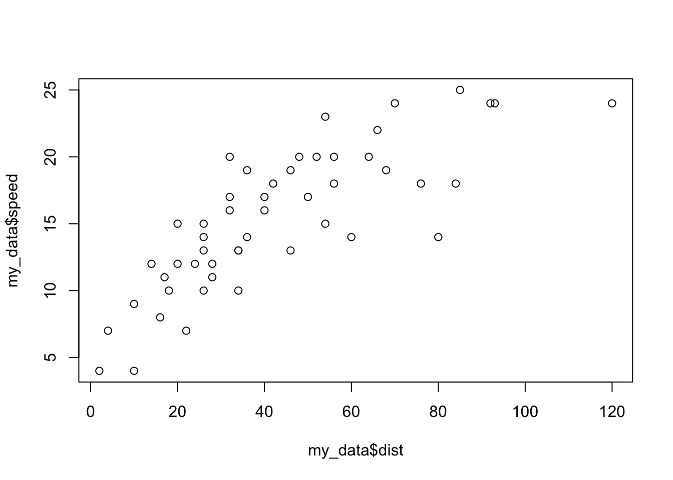
Let’s briefly explore another, related element of R Markdown: displaying plots. We’ll plot car speed as a function of distance (Y as a function of X).

# Plotting speed vs. distance from the cars data set
plot(my_data$speed ~ my_data$dist)

Awesome! We can see our code and our plot output.

Running code in R Markdown

I’ve been pressing the “Knit” button to see the output of my code, but you can also run your code in RStudio as if you’re doing it in a normal R script. You can just put your cursor wherever you want and then press command + return on a Mac, or control + Enter on a PC.

As you run the code in R Markdown, the output will appear below your code chunk:

Running your code within the code chunk first (instead of knitting it) is especially useful if you want to work through any errors, since the error messages will be easier to understand.

There’s also a neat trick you can use to make sure you’ve run all the necessary code and prevent errors. Pressing the button in the image below will run all of the code up to the chunk that you’re on, so you don’t have to manually go line by line or chunk by chunk.

Changing your R Markdown theme

One last thing you can do to make your document look nice is to change the theme. You can click on the gear icon in the toolbar at the top, and select “Output Options…”

A window will open up, from which you can do things like change the theme of your HTML document. If you go to “Apply theme” and select the dropdown menu, you’re given a list of different themes to choose from. Changing the theme will do things like change the fonts and colors that are displayed. You can play around with the themes to see what you prefer, just remember to press “Knit” to process the theme change.

If you’re interested in HTML and CSS, you can also apply your own CSS file to change the style of the document. Again, we’re going to keep it simple in this blog post—you can explore CSS on your own but please comment down below if you have any cool style sheets/themes for your R Markdown documents.

In the same way that you can change the theme of your document, you can also change the syntax highlighting. That changes how your code looks when it’s embedded in the document. For example, the image below shows the “zenburn” option.

Now it’s time for what I think is the most useful addition. The “Output Options” window also allows you to include an interactive, clickable table of contents for your document. This is especially useful for larger documents with multiple sections. The table of contents in your document will be based off of the different headings that you use, with smaller heading sizes nested within larger ones.

You’ll notice that headings 4, 5, and 6 aren’t included in the table of contents. You can change this if you want in the “Output Options” window, where it says “depth of headers for table of contents”. If you set the depth of the headings to 6, then the table of contents will display headings all the way up to heading level 6.

Once you make these changes, you’ll notice that these changes have also been added to the heading section of your document. This means that once you familiarize yourself with the themes, you can type this information into the heading yourself. I showed you how to do it via “Output Options” because we didn’t know what the different themes were called, nor what our options were.

One quick pointer for creating an R Markdown document is to end your document with the code sessionInfo(). This will show the information about your current R session, including the version of R you’re using, the operating system, and the packages you have loaded up. The reason this is important is because packages and software get updated over time and things can change. Certain aspects of your code might not work in the same way in the future, depending on what versions of software and packages you’re using. Having that information in the future can help you track down the issues. If you know the version information for how the code was originally run, then there are ways to download older versions of R and associated packages, or at least know where the error stems from (and how to fix it in the code). In essence, including your session info can help ensure reproducibility in the future.

sessionInfo()

## R version 4.2.2 (2022-10-31)
## Platform: x86_64-apple-darwin17.0 (64-bit)
## Running under: macOS Big Sur ... 10.16
## 
## Matrix products: default
## BLAS:   /Library/Frameworks/R.framework/Versions/4.2/Resources/lib/libRblas.0.dylib
## LAPACK: /Library/Frameworks/R.framework/Versions/4.2/Resources/lib/libRlapack.dylib
## 
## locale:
## [1] en_US.UTF-8/en_US.UTF-8/en_US.UTF-8/C/en_US.UTF-8/en_US.UTF-8
## 
## attached base packages:
## [1] stats     graphics  grDevices utils     datasets  methods   base     
## 
## loaded via a namespace (and not attached):
##  [1] bookdown_0.31    digest_0.6.31    R6_2.5.1         lifecycle_1.0.3 
##  [5] jsonlite_1.8.4   magrittr_2.0.3   evaluate_0.19    highr_0.9       
##  [9] blogdown_1.16    stringi_1.7.8    cachem_1.0.6     rlang_1.0.6     
## [13] cli_3.4.1        rstudioapi_0.14  jquerylib_0.1.4  bslib_0.4.2     
## [17] vctrs_0.5.1      rmarkdown_2.19.1 tools_4.2.2      stringr_1.5.0   
## [21] glue_1.6.2       xfun_0.35        yaml_2.3.6       fastmap_1.1.0   
## [25] compiler_4.2.2   htmltools_0.5.4  knitr_1.41       sass_0.4.4

And that’s it for our basic R Markdown tutorial! You learned how to create an R Markdown document, how to apply different types of text formats, how to embed code inline or in code chunks, and how to stylize your final R Markdown document. Our next blog post will be about how to use R Markdown to learn R, so keep your eyes peeled for a Part Two.

Have any cool R Markdown documents you’ve created? Share links in the comments below! 👇